gnuplot Templates

=========Start_Up======================

donsauer$ cd /Users/donsauer/Downloads/gnuplot-4.2.4/demo 

donsauer$ gnuplot

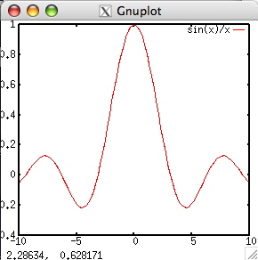
gnuplot>  plot sin(x)/x   

=========Functions_And_Variables======================

print pi

comb(n,k) = n!/(k!*(n-k)!)

print comb(5,4)

min(a,b) = (a < b) ? a : b

print min(5,3)

w = 2

q = floor(tan(pi/2 - 0.1))

f(x) = sin(w*x)

sinc(x) = sin(pi*x)/(pi*x)

delta(t) = (t == 0)

ramp(t) = (t > 0) ? t : 0

comb(n,k) = n!/(k!*(n-k)!)

len3d(x,y,z) = sqrt(x*x+y*y+z*z)

plot f(x) = sin(x*a), a = 0.2, f(x), a = 0.4, f(x)

file = "mydata.inp"

file(n) = sprintf("run_%d.dat",n)

`rand(0)` returns a pseudo random number in the interval [0:1] 

`rand(-1)` resets both seeds to a standard value.

`rand(x)` for x>0 sets both seeds to a value based on the value of x.

`rand({x,y})` for x>0 sets seed1 to x and seed2 to y.

f(x) = 0<=x && x<1 ? sin(x) : 1<=x && x<2 ? 1/x : 1/0

print f(.5)

=========Math_Terms======================

**   a**b exponentiation

*     a*b multiplication

/     a/b division

%    a%b * modulo

+    a+b addition

-     a-b subtraction

==  a==b equality

!=   a!=b inequality

<    a<b less than

<=  a<=b less than or equal to

>    a>b greater than

>=  a>=b greater than or equal to

&    a&b * bitwise AND

^    a^b * bitwise exclusive OR

|     a|b * bitwise inclusive OR

&&  a&&b * logical AND

||    a||b * logical OR

.     A.B string concatenation

eq  A eq B string equality

ne  A ne B string inequality

=========Pause======================

pause -1 "Hit return to continue"

pause 10 "Isn't this pretty? It's a cubic spline."

pause mouse "Click any mouse button on selected data point"

=========Mouse_Terms======================

When mousing is active, clicking in the active window will set several user variables

in MOUSE X MOUSE Y MOUSE X2 and MOUSE Y2

gnuplot> pause mouse 

         print  MOUSE_X , MOUSE_Y

gnuplot> print  MOUSE_X , MOUSE_Y

987652.839223448 -100.379746835443

=========LogGraphs======================

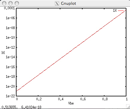
set xrange [0:1]

set log y

set xlabel "Vbe" offset -3,-2

set ylabel "IE" offset   3,-2

plot 1e-21*exp(x/.026) title "NPN_1X"

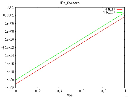
set title "NPN_Compare"

set xrange [0:1]

set log y

set xlabel "Vbe" offset -3,-2

set ylabel "IE" offset   3,-2

plot 1e-21*exp(x/.026) title "NPN_1X",1e-20*exp(x/.026) title "NPN_10X"

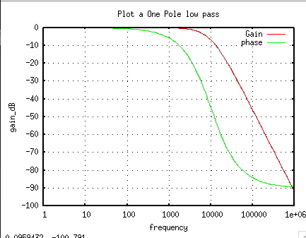
=========Grids======================

set title "Plot a One Pole low pass"

set xrange [1:1e6]

f = 10000

set log x

unset log y

set grid

set xlabel "frequency"

set ylabel "gain_dB"

plot 20*log(1/sqrt( 1+ (x/f)**2)) title "Gain", \

-180*atan( (x/f))/pi title "phase"

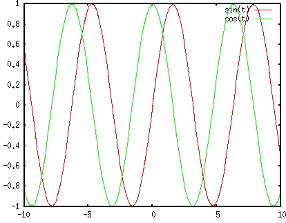
=========Dummy======================

independent, or "dummy", variable is "x"   or "t" if in parametric or polar mode

for the splot command are  "x" and "y"    or  "u" and "v" in parametric mode

set dummy t

plot sin(t), cos(t)

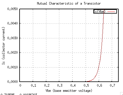
=========Dummy_And_Functions======================

# Bipolar Transistor (NPN) Mutual Characteristic

Ie(Vbe)=Ies*exp(Vbe/kT_q)

Ic(Vbe)=alpha*Ie(Vbe)+Ico

alpha = 0.99

Ies = 4e-14

Ico = 1e-09

kT_q = 0.025

set dummy Vbe

set grid

set offsets

unset log

unset polar

set samples 160

set title "Mutual Characteristic of a Transistor"

set xlabel "Vbe (base emmitter voltage)"

set xrange [0 : 0.75]

set ylabel "Ic (collector current)"

set yrange [0 : 0.005]

set key box

set key at .2,.0045

set format y "%.4f"

plot Ic(Vbe)

set format "%g"

provide a mechanism to put a boundary around the data inside of an autoscaled graph.

set offsets <left>, <right>, <top>, <bottom>

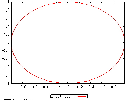
=========Parametric======================

2-d parametric function, plot sin(t),cos(t) draws a circle

3-d plotting, the surface is described as x=f(u,v), y=g(u,v), z=h(u,v).  

cos(u)*cos(v),cos(u)*sin(v),sin(u)  draws a sphere

set parametric

set dummy t

set autoscale

set samples 160

set title ""

set key box

set key below

plot sin(t),cos(t)

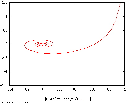
set autoscale x

set yrange [-1.5:1.5]

set trange [0.0001:10*pi]

plot sin(t)/t,cos(t)/t

show parametric  

    parametric is ON

unset parametric

=========Multiplot======================

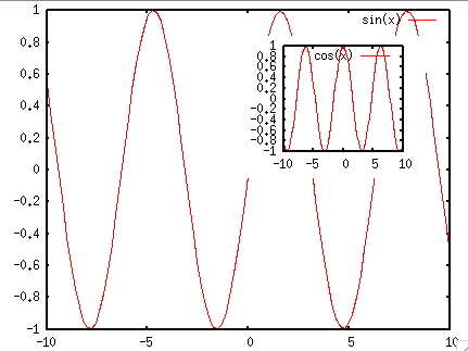
set multiplot

plot sin(x)

set origin 0.5,0.5

set size 0.4,0.4

clear

plot cos(x)

unset multiplot

=========MultiTrace======================

reset

set style function lines

set size 1.0, 1.0

set origin 0.0, 0.0

set multiplot

set size 0.5,0.5

set origin 0.0,0.5

set grid

unset key

set angles radians

set samples 250

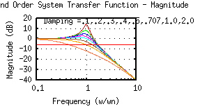
#  Plot Magnitude Response

set title "Second Order System Transfer Function - Magnitude"

mag(w) = -10*log10( (1-w**2)**2 + 4*(zeta*w)**2)

set dummy w

set logscale x

set xlabel "Frequency (w/wn)"

set ylabel "Magnitude (dB)" offset 1,0

set label 1 "Damping =.1,.2,.3,.4,.5,.707,1.0,2.0" at .14,17

set xrange [.1:10]

set yrange [-40:20]

plot \

  zeta=.1,mag(w), \

  zeta=.2,mag(w), \

  zeta=.3,mag(w), \

  zeta=.4,mag(w), \

  zeta=.5,mag(w), \

  zeta=.707,mag(w), \

  zeta=1.0,mag(w), \

  zeta=2.0,mag(w),-6

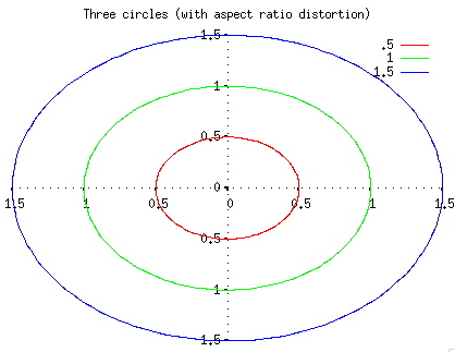
=========Polar======================

unset border

set clip

set polar

set xtics axis nomirror

set ytics axis nomirror

set samples 160

set zeroaxis

set trange [0:2*pi]

set title "Three circles (with aspect ratio distortion)"

plot .5,1,1.5

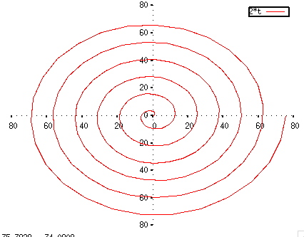
set trange [0:12*pi]

plot 2*t

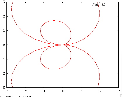
set polar

plot t*sin(t)

plot [-2*pi:2*pi] [-3:3] [-3:3] t*sin(t)

=========Complex======================

Can Define a complex function as so

compl(a,b)=a*{1,0}+b*{0,1}

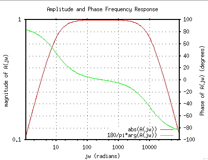
# amplitude frequency response

A(jw) = ({0,1}*jw/({0,1}*jw+p1)) * (1/(1+{0,1}*jw/p2))

p1 = 10

p2 = 10000

set dummy jw

set grid x y2

set logscale xy

set log x2

unset log y2

set key default

set key bottom center box

set title "Amplitude and Phase Frequency Response"

set xlabel "jw (radians)"

set xrange [1.1 : 90000.0]

set x2range [1.1 : 90000.0]

set ylabel "magnitude of A(jw)"

set y2label "Phase of A(jw) (degrees)"

set ytics nomirror

set y2tics

set tics out

set autoscale  y

set autoscale y2

plot abs(A(jw)), 180/pi*arg(A(jw)) axes x2y2

=========Load_data_File======================

      # This file is called   force.dat

      # This file needs LF convert Mac->PC

      # Force-Deflection data for a beam and a bar

      # Deflection    Col-Force       Beam-Force 

      0.000              0              0    

      0.001            104             51

      0.002            202            101

      0.003            298            148

      0.0031           290            149

      0.004            289            201

      0.0041           291            209

      0.005            310            250

      0.010            311            260

      0.020            280            240

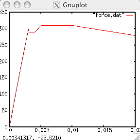
gnuplot> plot  "force.dat"

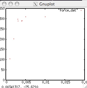
gnuplot> plot  "force.dat" with lines

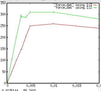
plot "force.dat" using 1:3 with linespoints ,"force.dat" using 1:2 with linespoints

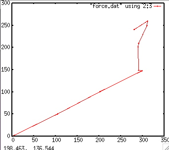
plot "force.dat" using 2:3 with linespoints 

gnuplot> show pointsize

pointsize is 1

gnuplot> set pointsize 6

=========ScriptFile======================

     # Gnuplot script file for plotting data in file "force.dat"

      # This file is called   force.p

      set   autoscale                        # scale axes automatically

      unset log                              # remove any log-scaling

      unset label                            # remove any previous labels

      set xtic auto                          # set xtics automatically

      set ytic auto                          # set ytics automatically

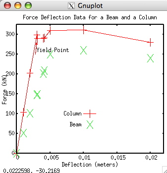
      set title "Force Deflection Data for a Beam and a Column"

      set xlabel "Deflection (meters)"

      set ylabel "Force (kN)"

      set key 0.01,100

      set label "Yield Point" at 0.003,260

      set arrow from 0.0028,250 to 0.003,280

      set xr [0.0:0.022]

      set yr [0:325]

      plot    "force.dat" using 1:2 title 'Column' with linespoints , \

              "force.dat" using 1:3 title 'Beam' with points

=========Line_Format======================

Style

set style data <style>

show style function

show style data

set style arrow <n> <arrowstyle>

set style fill <fillstyle>

set style histogram <histogram style options>

set style line <n> <linestyle>

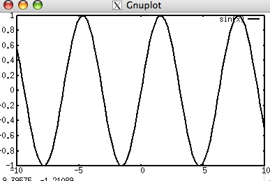
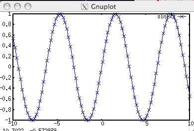
plot sin(x) lt -1 # black   {{linetype | lt <line_type>}

plot sin(x) lt 1   # red

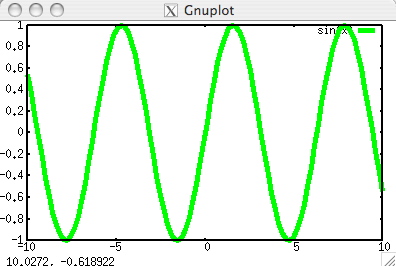
plot sin(x) lt 2   # green    

plot sin(x) lt 3   # blue 

plot sin(x) lt 4   # violet 

plot sin(x) lt 5   # cyan 

plot sin(x) lt 6   # brown

plot sin(x) lt 7   # orange 

plot sin(x) lt 8   # green

plot sin(x) lt -1 # black   

plot sin(x)  lt 2 lw 5 #   {linewidth | lw <line_width>}

 with lines, points, linespoints, impulses, dots, steps, fsteps, histeps, error-bars, labels, 

xerrorbars, yerrorbars, xyerrorbars, errorlines, xerrorlines, yerrorlines, xyerrorlines, boxes, 

histograms,  lledcurves, boxerrorbars, boxxyerrorbars,  nancebars, candlesticks, vectors, image, rgbimage or pm3d. 

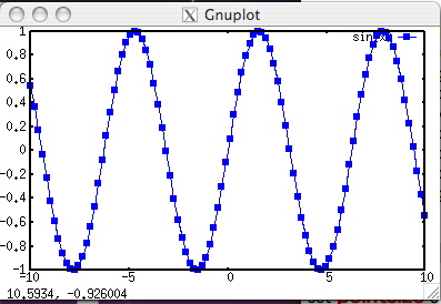
plot sin(x) with linespoints lt 3 pt 5 ps 3 # {pt <point_type>} {ps <point_size>}

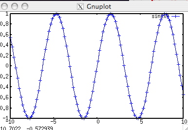
plot sin(x) with linespoints lt 3 pt 1 ps 3 

plot sin(x) with linespoints lt 3 pt 2 ps 3 #

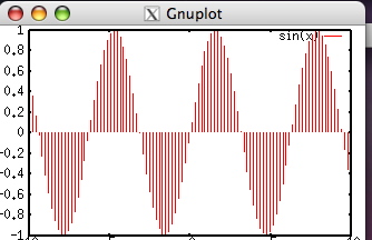
plot sin(x) with impulses

reset

set samples 25        # default, sampling is set to 100 points

unset xtics           # set xtics (0.002,0.004,0.006,0.008) changes tickmarks

unset ytics

set yrange [0:120]

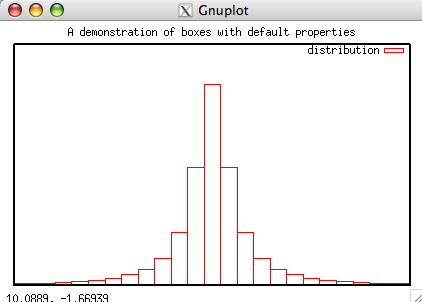
set title "A demonstration of boxes with default properties"

plot [-10:10] 100/(1.0+x*x) title 'distribution' with boxes

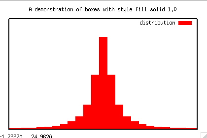
set title "A demonstration of boxes with style fill solid 1.0"

set style fill solid 1.0

replot

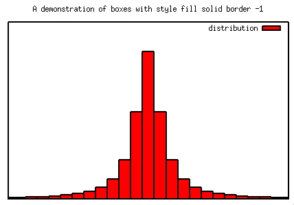
set title "A demonstration of boxes with style fill solid border -1"

set style fill solid border -1

replot

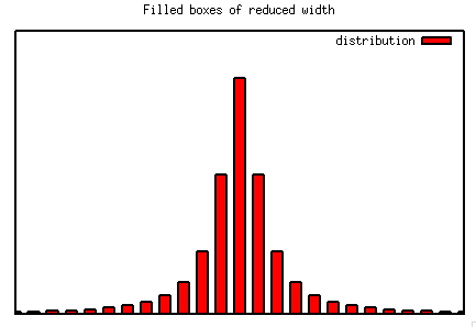
set title "Filled boxes of reduced width"

set boxwidth 0.5 

replot

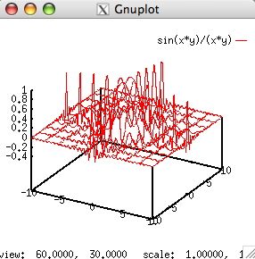
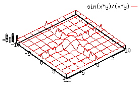
=========Surface_Plots======================

gnuplot> splot sin(x*y)/(x*y)

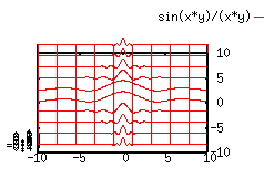
set view 10, 0, 1, 1

splot sin(x*y)/(x*y)

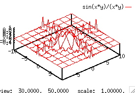
set view 10, 50, 1, 1

splot sin(x*y)/(x*y)

set view 30, 50, 1, 1

splot sin(x*y)/(x*y)

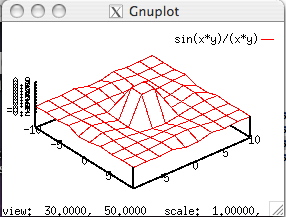
set hidden3d

set view 30, 50, 1, 1

splot sin(x*y)/(x*y)

set hidden3d

set view 100, 50, 1, 1

splot sin(x*y)/(x*y)

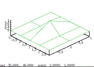
=========Plot_3D_File======================

# This file is called   glass3.dat

# This file needs LF convert Mac->PC

# x    y    z

 -1   -1    0

  0   -1    0 

  1   -1    0

  2   -1    0

  3   -1    0

 -1    0    0

  0    0    0 

  1    0    1

  2    0    0

  3    0    0

 -1    1    0

  0    1    0 

  1    1    0

  2    1    0

  3    1    0

set hidden3d

unset key

set style data line

set view 30,46

splot "glass3.dat"

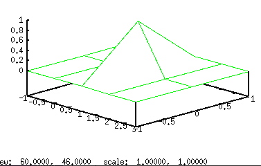
set hidden3d

unset key

set style data line

set view 60,46, 1,1

splot "glass3.dat"

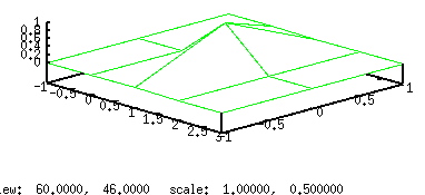
set hidden3d

unset key

set style data line

set view 60,46, 1,.5

splot "glass3.dat"

=========Formats======================

=========Other_Examples======================

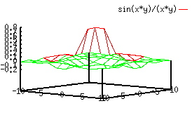
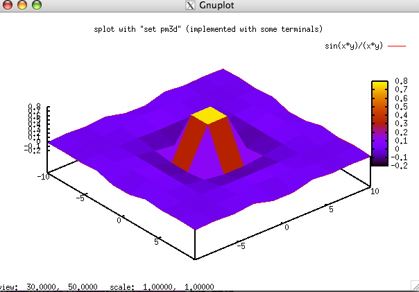
set pm3d

set hidden3d

set sample 3,3

set view 30, 50, 1, 1

splot sin(x*y)/(x*y)

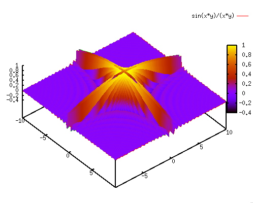
set hidden3d

set isosamples 101

set view 30, 50, 1, 1

splot sin(x*y)/(x*y)

set xtics autofreq

set ytics autofreq

set xrange [-1:1]

set yrange [-1:1]

set samples 51

set isosample 21

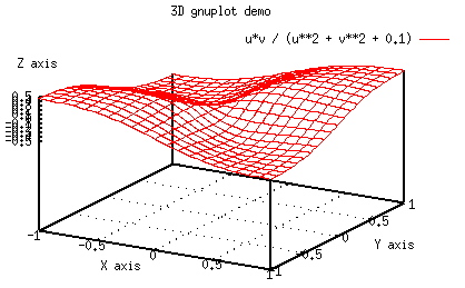
set dummy u,v

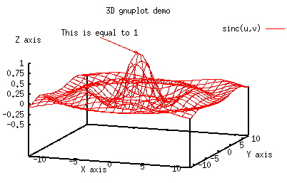
set title "3D gnuplot demo"

splot u*v / (u**2 + v**2 + 0.1)

splot [x=-3:3] [y=-3:3] sin(x) * cos(y)

pause -1 "Hit return to continue (12)"

set zrange [-1.0:1.0]

replot

pause -1 "Hit return to continue (13)"

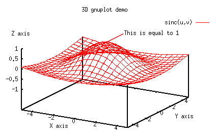
set title "Sinc function"

set zrange [-1:1]

set label 1 "This is equal to 1" at 0,3.2,1 left

set arrow 1 from 0,3,1 to 0,0,1

sinc(u,v) = sin(sqrt(u**2+v**2)) / sqrt(u**2+v**2)

splot [-5:5.01] [-5:5.01] sinc(u,v)

set view 70,20,1

set zrange [-0.5:1.0]

set ztics -1,0.25,1

set label 1 "This is equal to 1" at -5,-2,1.5 centre

set arrow 1 from -5,-2.1,1.4 to 0,0,1

splot [-12:12.01] [-12:12.01] sinc(u,v)